1 Introduction
Classical biplots are representations of multivariate datasets. Datasets can be organized in many ways. A consistent way to organize the data is called tidy data (Wickham 2014). A tidy data matrix is characterized by three rules:
- Each variable must have its own column.
- Each sample must have its own row.
- Each value must have its own cell.
Biplots can be used to look at the tidy data matrix with information on both the samples and the variables. The common presentation of variables (usually by arrows) and samples allows both the interpretation of sample cluster and in addition relations between variables and objects can be described.
Despite the widespread use of biplot there a some discussions about the correct presentation and interpretation of biplot:
John C. Gower (2003): … some of the faults often found in published biplot diagrams:
- unequal scaling of the axes
- use of E-formats
- ugly scale divisions
- no scales on biplot axes
- one-standard error lengths of vectors
- item scales given unnecessarily for canonical axes and no scales for the original variables
- item separate canonical scales for samples and for variables.
Some of these faults are also present using standard biplots in R (e.g. biplot with prcomp).
Any multivariate data matrix contain information on two distinct entities, the rows and the columns. We restrict to the situation where rows correspond to the units sampled or observed, and columns correspond to variables measured on these units (tidy data).
By looking at the raw data, it is not possible to understand the relationship between the variables or to see some structure in the sampled units. The humain brain has not evolved to interpret tables of numbers in this way. We are much better in absorbing pictorial information.
A biplot is a representation of the rows and the columns of a data matrix in a joint display with few dimensions (The bi- in biplots is related to these entities). The aim of a biplot is to make data more transparent, and to assist in the interpretation of structures and patterns.
2 Exact Euclidean Biplot
Biplot is an approach to statistical graphics for large tables of data. This methodology is a generalization of the scatterplot of two variables to the case of many variables. The essential property of all biplots is the two modes (rows and columns of the table or samples and variables) not the dimension of the plot. We will be mainly concerned with two-dimemsional biplots although one- or three- dimensional plots are possible.
An exact biplot’s defintion seems to be not so easy (see Amazon Customer Reviews of (Gower et al. 2011): Understanding biplots is motivated by the fact that most of the available literature on the topic is not accessible to many who would benefit from these techniques. Unfortunately this books falls (backwards) into that selfsame category. The first chapter tells us that Biplots have been around at least the 17th century. And, that they go by a wide variety of names. And, have at least two main types. But, it never tells us what a bi-plot is.
Two steps are essential for the the construction of biplots - one step step is universally valid for all types of biplots (the definition of a biplot), another step depends on the appropriate distance and the criteria used to get an appropriate approximation of the data.
2.1 Decomposition - innerproduct of biplot vector and biplot points
Biplots are defined as the decomposition of a target matrix with dimension \(n \times p\) into a product of two matrices, called left and right matrix with \(n \times 2\) and \(2 \times p\) dimensions, so that
                    target matrix = left matrix * right matrix
                    S = X * Y.
The following example is specified on p. 19 of Greenacre (2010). The content of the data matrix can be interpreted as values of four variables for a sample of 5 probands, e.g. results of a survey with rating scales for five products.
\[\mathbf{S} = \left[\begin{array} {rrr} 8 & 2 & 2 & -6 \\ 5 & 0 & 3 & -4 \\ -2 & -3 & 3 & 1 \\ 2 & 3 & -3 & -1\\ 4 & 6 & -6 & -2 \end{array}\right]\]
The left and right matrix of a possible decomposition (decomp1) are shown in the following tables.
\[\mathbf{S} = \left[\begin{array}{rrr}2&2 \\1&2 \\-1&1 \\1&-1 \\2&-2 \\\end{array}\right] \times \left[\begin{array}{rrr}3&2&-1&-2 \\1&-1&2&-1 \\\end{array}\right]\]
The biplot can be constructed ploting the rows of the left matrix (as points) and the columns of the right matrix (as arrows). The next figure shows these biplot points (black, left matrix) and biplot vectors (red, right matrix).
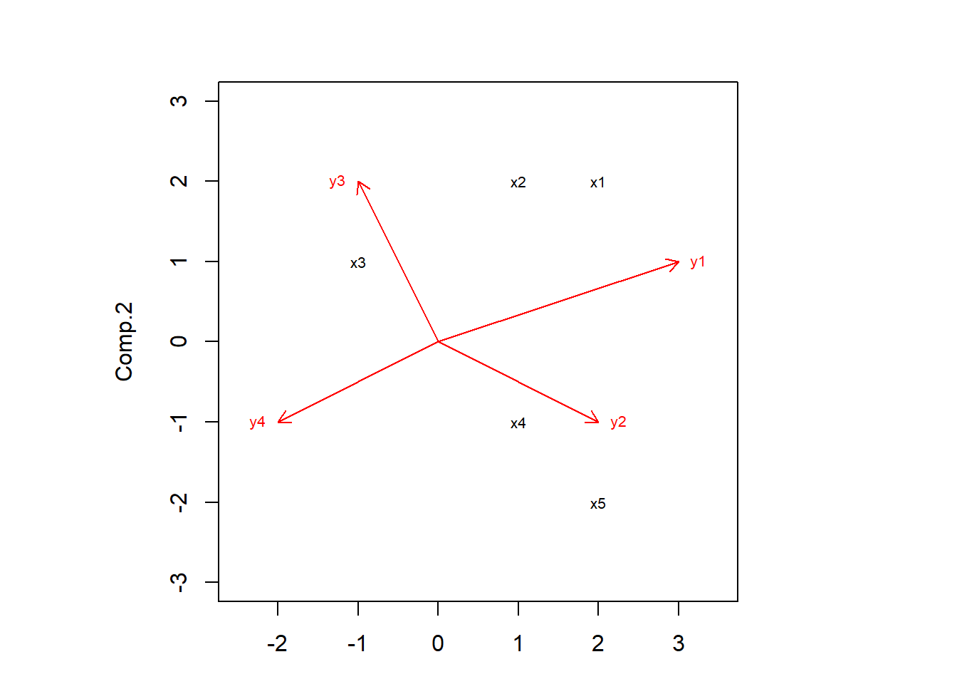
In this way two sets of points are graphed in a joint plot, according to coordinates provided by the decomposition of a target matrix.
The usefulness of biplots as a method of data visualization is based on a specific geometric interpretation of the scalar product. The scalar product of two vectors is defined as the sum of cross-products (see for an introduction to linear algebra with R (Hojsgaard 2015). The geometric interpretation of the scalar product of a biplot point and a biplot vector is the projection of the first point onto the vector. The biplot points can be projected onto the biplot axes, and their projections are proportional to the scalar products which are equal to the target matrix (see next Figure). All biplots have this property, the property is inherent to the definition of the biplot.
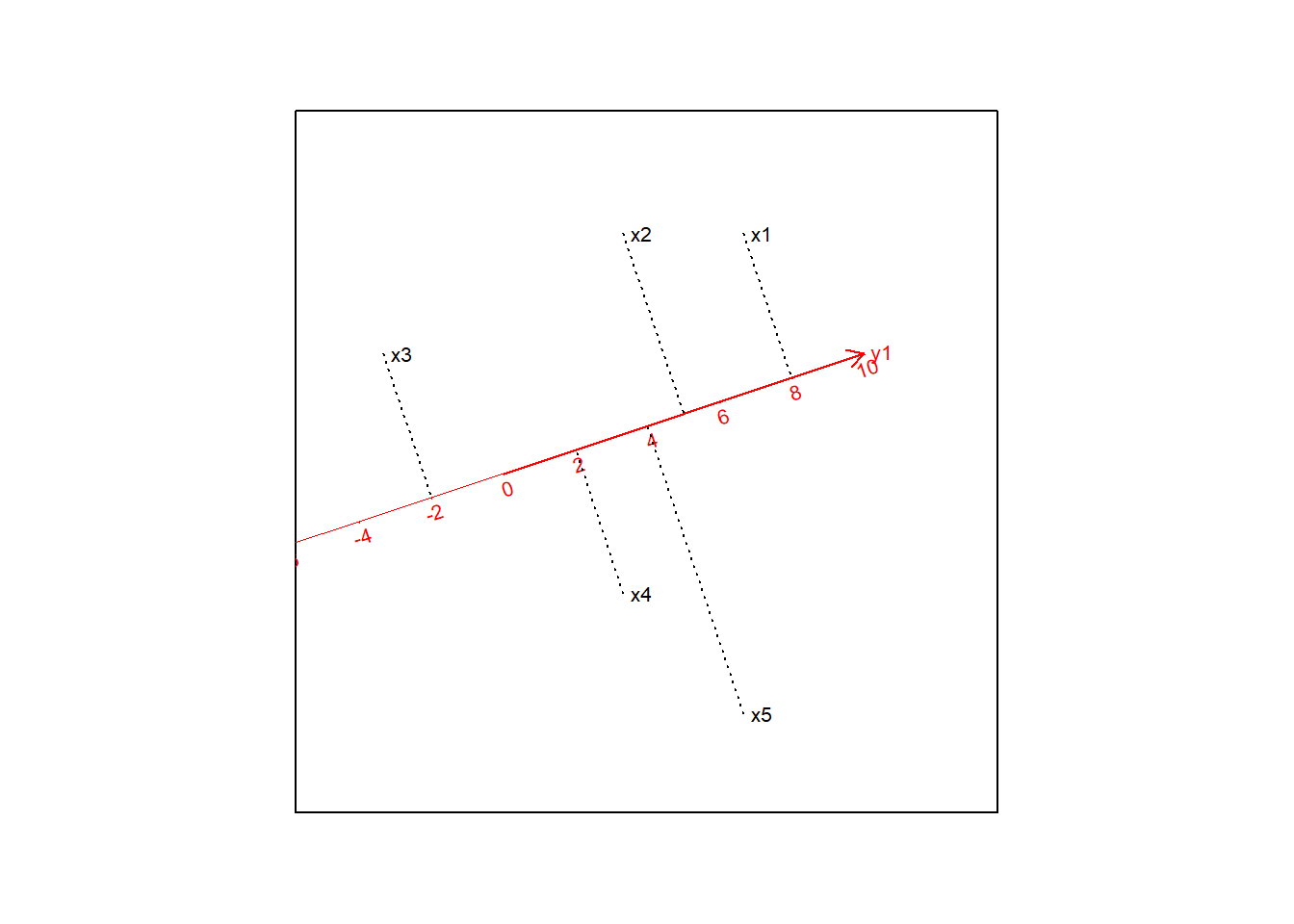
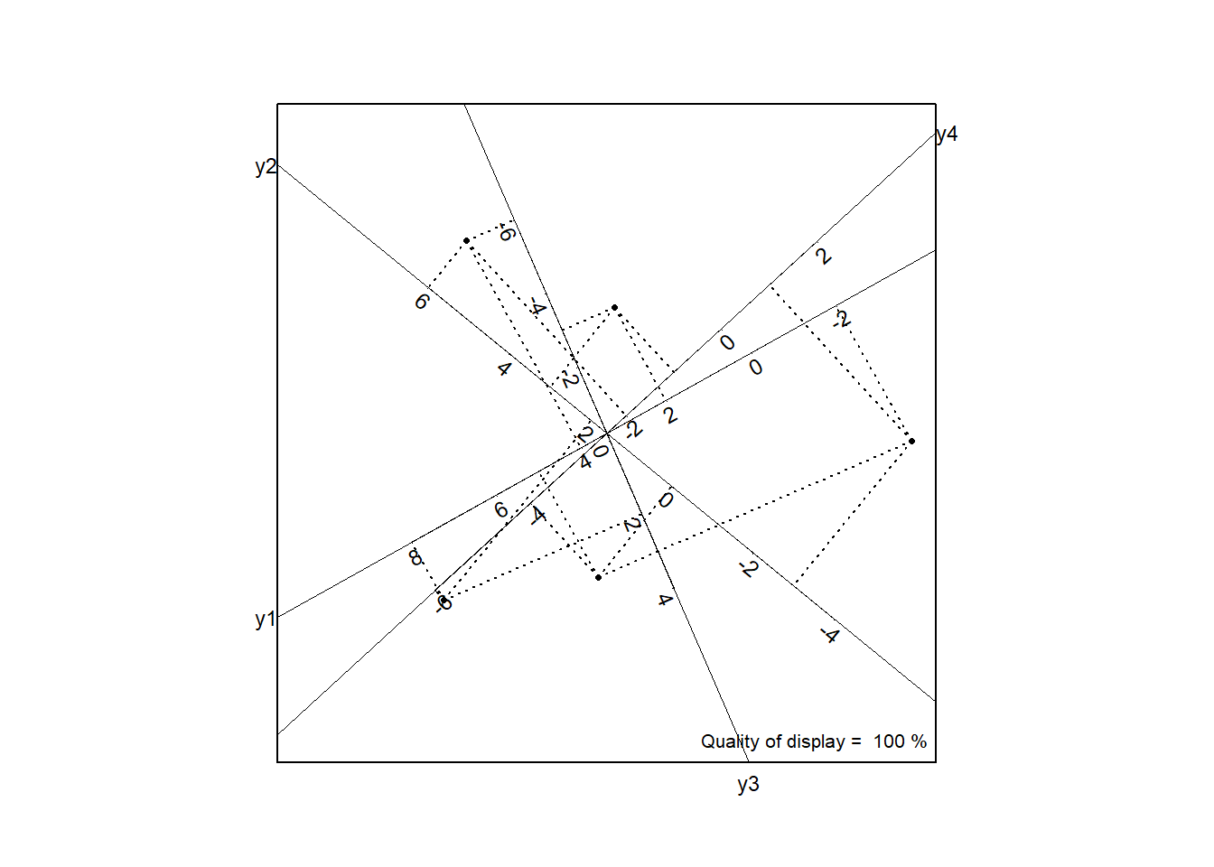
The practical value of the biplot property of representing data by scalar products is only truly apparent if one thinks of the biplot axes as beeing calibrated. This is the placing of tic marks on the biplot axes indicating a scale for reading of the values in the target matrix by simply projecting the biplot points onto the biplot axes. Next Figure shows one axis (y1) in a calibrated form. With this figure we can see the values of the first column of the target matrix (8,5,-2,2,4).
The fact that axes can be calibrated gives the raison d’être of the biplot’s interpretation.
Rather than dealing with latent variables, biplot offer the complementary approach of representing the original variables. The axes representing the latent variables (in standard biplots often labelled with PC1 and PC2) will not be shown; they form only what may be regarded as scaffolding axes on which the biplot is built.
2.2 Euclidean distance preserving - innerproduct of Biplot points
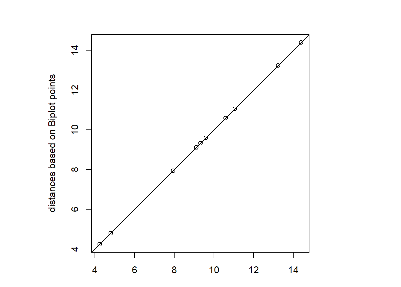
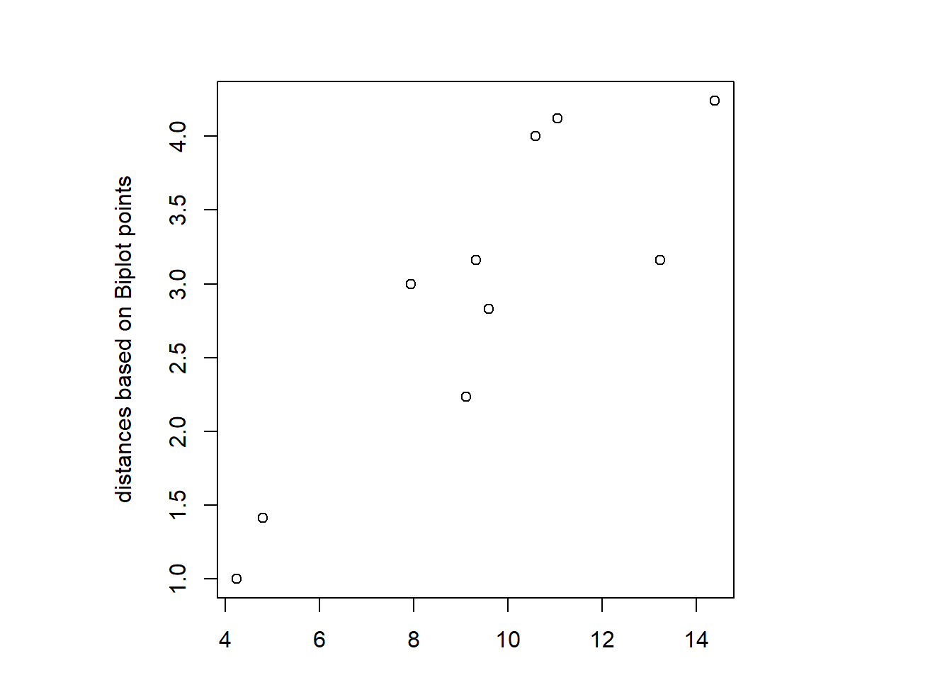
The decomposition in the previous chapter is not unique. For an exact Euclidean Biplot we postulate a second principle: the Euclidean distance matrix for the points of the target matrix should be identical to the distance matrix of the Biplot points.
Next Figure compares the distance matrices for the previous decomposition (decomposition 1). It can be seen that the second condition is not fullfilled.
Here is another decomposition of the target matrix S (decomposition 2):
\[S = \left[\begin{array}{rrr}-9.37&-4.49 \\-5.14&-4.85 \\3.77&-2.97 \\-3.77&2.97 \\-7.54&5.93 \\\end{array}\right] \times \left[\begin{array}{rrr}-0.73&-0.43&0.17&0.5 \\-0.26&0.46&-0.8&0.3 \\\end{array}\right]\]
Based on decomposition 2 the distances between biplot points (matrix X) are identical to the distances between the original points (target matrix) - see Figure 5 ).
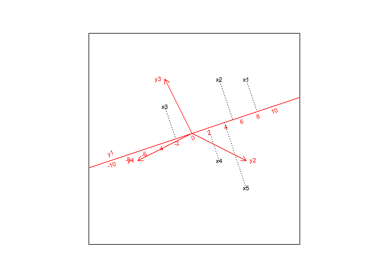
The calibratred biplot based on this decomposition is shown in Figure 6 together with the original data matrix. Each cell in the target matrix can be identified in the calibrated biplot,
| y1 | y2 | y3 | y4 | |
|---|---|---|---|---|
| x1 | 8 | 2 | 2 | -6 |
| x2 | 5 | 0 | 3 | -4 |
| x3 | -2 | -3 | 3 | 1 |
| x4 | 2 | 3 | -3 | -1 |
| x5 | 4 | 6 | -6 | -2 |
2.3 Construction of an Exact Euclidean Biplot
Two conditions have to be fullfilled:
- the target matrix S with dimension \(n \times p\) can be decomposited into a product of two matrices X and Y with \(n \times 2\) and \(2 \times p\) dimensions
- the Euclidean distance is preserved
2.3.1 Singular value decomposition
The singular value decomposition (SVD) is a fundamental tool in statistics. One of the most useful results in matrix theory solves the problem to find a best approximation k-dimensional linear subspace, i.e. to find a matrix of lower rank k that resembles the target matrix as closely as possible.
The basic result of SVD is as follows: any rectangular n x p matrix Y can be expressed as the product of three matrices: \[Y = U*D*t(V)\] where U is a n x r, V is p x r and D is a r x r diagonal matrix with positive numbers on the diagonal in descending order (r = rank of Y).
2.3.2 Exact Euclidean Biplot for matrices with rank 2
The singular value decomposition provide the solution in exactly the form that is required for the exact euclidean biplot if the rank of Y = 2. Then D is a 2 x 2 diagonal matrix and the matrix of biplot points is U*D and of biplot vectors is t(V) with \(n \times 2\) and \(2 \times p\) dimensions respectively. The Euclidean distance is preserved. Decomposition 2 in chapter 2.2 is calculated with this singular value decomposition.
The problem with the biplot definition in chapter 2 is that an exact decomposition of the target matrix is only possible if there are only two variables or the rank of the target matrix is 2 (as in the example in 2.2). In practice however no large matrix is of low rank. The idea is to lessen the stipulation of preserving the Euclidean distance to finding the best approximating 2-dimensional linear subspace which minimizes the sum of the sqared distances.
3 Best approximating Euclidean Biplot
3.1 example data
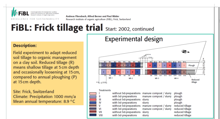
To demonstrate the construction of calibrated biplots for tidy data with rank > 2 we use empirical data from a field experiment to adapt reduced soil tillage to organic management on a clay soil. Reduced tillage means shallow tillage at 5 cm depth compared to ploughing at 15 cm depth. The complete design of the study is illustrated in Figure 7.
The empirical tidy data matrix has 16 rows (lots of land, labeled with O02, O04, O05, O07, O09, O11, O13, O16 and the correspondent lots on the opposite side w02, ,,, ,w16 according to the design of the trial) and 9 columns with the variables pH, Ctotal, Corg, Ntotal, Bulk, DOC, DON, Cmic, Nmic (see Figure 8).
| PlotCode | pH | Ctotal | Corg | Ntotal | Bulk | DOC | DON | Cmic | Nmic |
|---|---|---|---|---|---|---|---|---|---|
| O02 | 7.3 | 2.96 | 2.38 | 0.262 | 1.38 | 76.0 | 12.9 | 795.5 | 112.9 |
| O04 | 7.3 | 3.13 | 2.49 | 0.260 | 1.35 | 70.5 | 11.0 | 752.2 | 102.0 |
| O05 | 7.3 | 3.55 | 2.66 | 0.276 | 1.37 | 76.0 | 12.3 | 852.3 | 115.4 |
| O07 | 7.3 | 4.18 | 2.65 | 0.278 | 1.36 | 81.8 | 11.6 | 861.7 | 119.1 |
| O09 | 7.2 | 3.95 | 4.19 | 0.381 | 1.22 | 83.6 | 12.7 | 1200.8 | 177.9 |
| O11 | 7.1 | 4.13 | 4.40 | 0.387 | 1.17 | 98.7 | 13.7 | 1255.4 | 183.8 |
| O13 | 6.6 | 3.79 | 4.23 | 0.395 | 1.15 | 88.1 | 14.1 | 1116.0 | 144.3 |
| O16 | 6.7 | 3.98 | 4.46 | 0.417 | 1.12 | 106.3 | 15.1 | 1103.6 | 156.4 |
| W02 | 7.2 | 3.58 | 3.17 | 0.321 | 1.33 | 97.8 | 14.9 | 1104.2 | 171.0 |
| W04 | 7.2 | 3.78 | 3.23 | 0.327 | 1.35 | 82.3 | 14.6 | 1134.7 | 169.4 |
| W05 | 7.2 | 4.15 | 3.53 | 0.362 | 1.30 | 94.1 | 16.0 | 1208.9 | 189.7 |
| W07 | 7.3 | 4.35 | 3.04 | 0.309 | 1.33 | 93.7 | 14.5 | 1063.8 | 157.0 |
| W09 | 7.2 | 3.22 | 3.51 | 0.324 | 1.19 | 77.0 | 14.6 | 881.3 | 120.9 |
| W11 | 7.1 | 3.36 | 3.87 | 0.366 | 1.21 | 84.3 | 16.0 | 1052.1 | 147.0 |
| W13 | 6.8 | 3.25 | 3.81 | 0.365 | 1.23 | 77.1 | 13.2 | 900.1 | 127.2 |
| W16 | 6.6 | 3.29 | 3.87 | 0.363 | 1.18 | 73.1 | 16.8 | 828.5 | 108.2 |
The design of the study allows to explore the effect of reduces soil tillage by several statistical methods (e.g. pairwise comparison). Initially we do not incorporate the design information. We want to have a better look at the data to understand the relationship between the variables or to see some structure in the sampled units. A biplot is aimed to make data more transparent.
3.2 Singular value decomposition and calibrated biplot
Because the rank of the empirical data matrix is greater than 2, we can not construct an Exact Euclidean Biplot but only a Best approximating Euclidean Biplot. To get a best approximation in a 2 - dimensional subspace we can use a singular value decomposition by using only the first two columns of V and D of the SVD.
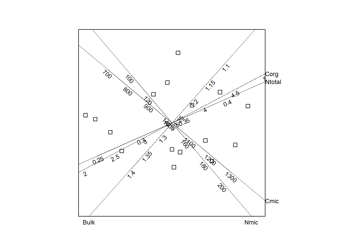
With left matrix Yl = U * D and right matrix Yr = V the joint plot of Yl and Yr can be constructed, Based on this decomposition as scaffolding axes the calibrated biplot for this data matrix with 16 rows (samples) and 9 columns (variables) is shown in Figure 9.
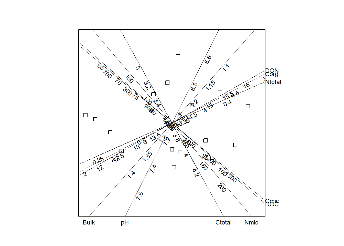
Three facts regarding calibrated should taken into account of a biplot’s interpretation.
- cross products between biplot points and biplot vectors equals matrix approximation (definition of biplot). The projection of a biplot point on a scaled biplot vector can be interpreted as approximative value of the correspondent variable.
Because projections are invariant with respect to rotation and orthogonal shifts of all biplot vectors.
cross products between biplot points (Euclidean distance between biplot points) equals Euclidean distance between original approximated points.
as a diagnostic tool for biplot vectors the so called adequacy is calculated for each variable. This parameter is proportional to the pearson correlation coefficient between the original and the approximated variable and therefore can be used to drop out variables which are insufficient represented by the chosen calculated approximation.
These correlation coefficients (adequacy) are shown in Figure 10.
| pH | Ctotal | Corg | Ntotal | Bulk | DOC | DON | Cmic | Nmic | |
|---|---|---|---|---|---|---|---|---|---|
| predictivity | 0.9201028 | 0.8528252 | 0.9694988 | 0.985822 | 0.9478525 | 0.8847224 | 0.6574206 | 0.9677073 | 0.9573185 |
3.3 Calibrated biplot with a reduced number of variables
Selecting six variables with the best predictivity values results in a the reduced biplot shown in Figure 11.
3.4 Rotated calibrated biplot
Because the presentation of a calibrated biplot is not unique some transformations can be applied to get a easier interpretation : here the biplot is rotated so that the biplot axis with the highest axis predictivity (Ntotal) is in a horizontal position.
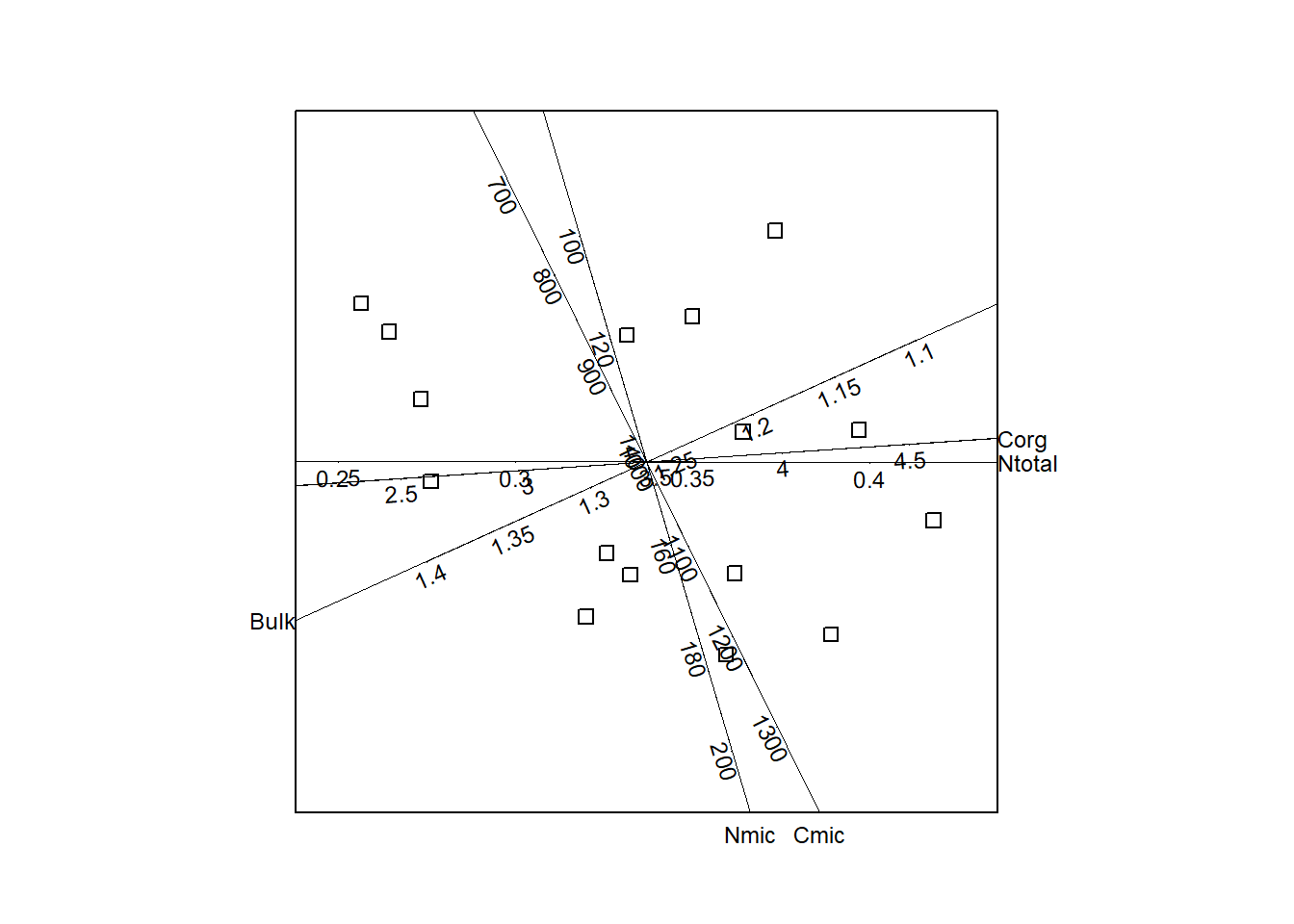
Just as orthogonal shift of some or all biplpot axes can be operated e.g. to have a better look at biplot points in the middle of the figure.
3.5 Calibrated biplot with labelled biplot points
Until now information about the study design (see Figure 7) is not used. In Figure 13 the calibrated biplot is shown with biplot points colored with respect to the experimantal design:
- darkred = south/plough
- red = north/plough
- darkgreen = south/reduced tillage
- green = north/reduced tillage
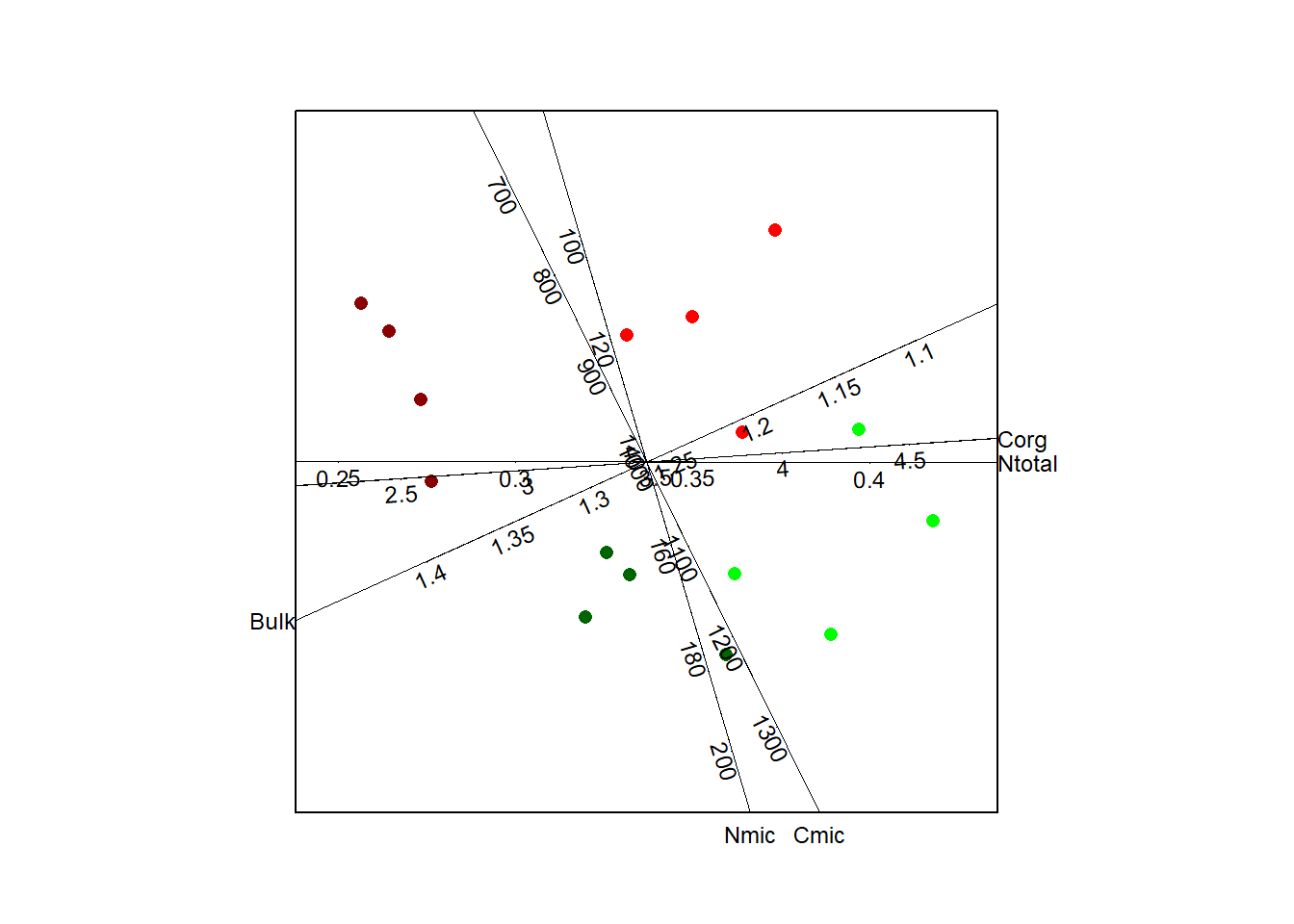
The four treatment groups are clearly separated by the PCA. In contrast to canonical variate analysis (CVA), PCA focuses not on observations grouped in K classes/treatments. Therefore the detected group separation shows some indication for an effect of the reduced soil tillage.
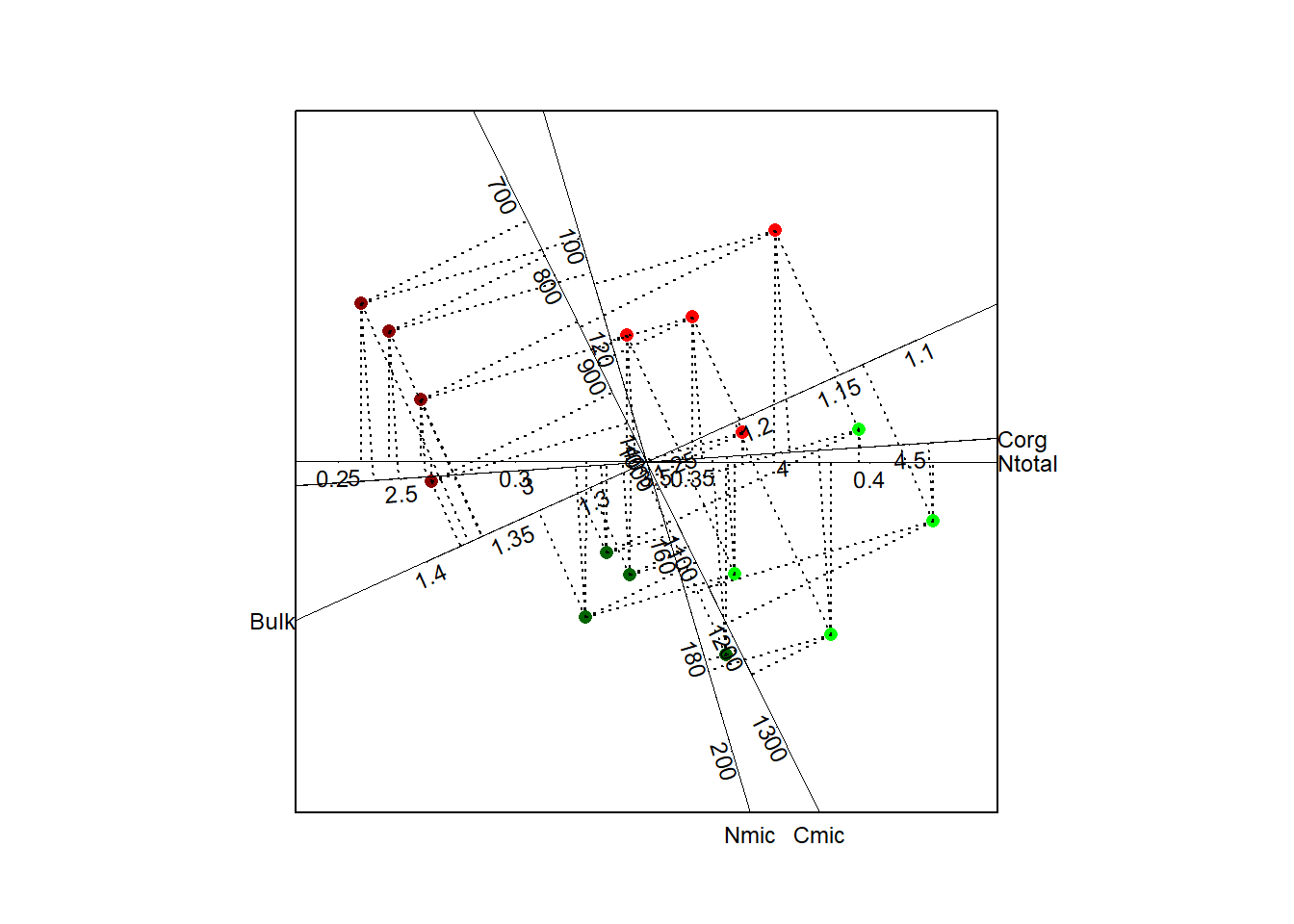
Looking at Figure 14 this effect can be described by higher carbon in microbial biomass (>1150) and higher nitrogen in microbial biomass (>140), This is valid for both regional different located compartments (south/north) which are characterized by a different soil bulk density (< 1.25 [mg/m3] south, > 1.25 [mg/m3] for the northern regions).
References
Gower, John. 2003. Unified Biplot Geometry. http://mrvar.fdv.uni-lj.si/pub/mz/mz19/gower.pdf.
Gower, John, Sugnet Lubbe, and Niëll le Roux. 2011. Understanding Biplots. Wiley. https://onlinelibrary.wiley.com/doi/pdf/10.1002/9780470973196.fmatter.
Greenacre, Michael. 2010. Biplot in Practice. FBBVA. https://www.fbbva.es/wp-content/uploads/2017/05/dat/DE_2010_biplots_in_practice.pdf.
Hojsgaard, Soren. 2015. Introductory Linear Algebra with R. http://bendixcarstensen.com/APC/linalg-notes-BxC.pdf.
Wickham, Hadley. 2014. Tidy Data. http://www.jstatsoft.org/v59/i10/paper.